A super quick, very practical, theory-free, hands-on intro to writing a simple classification model in R, using the caret package. If you want to skip the tutorial, you can find the R code here. Quick note: if the code examples look weird for you on mobile, give it a try on a desktop (you can’t do the tutorial on your phone, anyway!).
One of the biggest barriers to learning for budding data scientists is that there are so many different R packages for machine learning. Each package has different functions for training the model, different functions for getting predictions out of the model and different parameters in those functions. So in the past, trying out a new algorithm was often a huge ordeal. The caret package solves this problem in an elegant and easy-to-use way. Caret contains wrapper functions that allow you to use the exact same functions for training and predicting with dozens of different algorithms. On top of that, it includes sophisticated built-in methods for evaluating the effectiveness of the predictions you get from the model. I recommend that you do all of your machine-learning work in caret, at least as long as the algorithm you need is supported. There's a nice little intro paper to caret here.
Most of you have heard of a movie called Titanic. What you may not know is that the movie is based on a real event, and Leonardo DiCaprio was not actually there. The folks at Kaggle put together a dataset containing data on who survived and who died on the Titanic. The challenge is to build a model that can look at characteristics of an individual who was on the Titanic and predict the likelihood that they would have survived. There are several useful variables that they include in the dataset for each person:
For our purposes, machine learning is just using a computer to “learn” from data. What do I mean by “learn?” Well, there are two main different possible types of learning:
In order to follow this tutorial, you will need to have R set up on your computer. Here's a link to a download page: Inside R Download Page. I also recommend RStudio, which provides a simple interface for writing and executing R code: download it here. Both R and RStudio are totally free and easy to install.
Go ahead and open up RStudio (or just R, if you don't want to use RStudio). For this tutorial, you need to install the caret package and the randomForest package (you only need to do this part once, even if you repeat the tutorial later).
install.packages("caret", dependencies = TRUE)
install.packages("randomForest")
Now we have to load the packages into the working environment (unlike installing the packages, this step has to be done every time you restart your R session).
library(caret)
library(randomForest)
Go the Kaggle download page to find the dataset. Download train.csv and test.csv, and be sure to save them to a place you can remember (I recommend a folder on your desktop called “Titanic”). You might need to sign up for Kaggle first (you should be using Kaggle anyway!)
To load in the data, you first set the R working directory to the place where you downloaded the data.
setwd("FILE PATH TO DIRECTORY")
For example, I downloaded mine to a directory on my Desktop called Titanic, so I typed in
setwd("~/Desktop/Titanic/")
Now, in order to load the data, we will use the read.table function
trainSet <- read.table("train.csv", sep = ",", header = TRUE)
This command reads in the file “train.csv”, using the delimiter “,”, including the header row as the column names, and assigns it to the R object trainSet.
Let's read in the testSet also:
testSet <- read.table("test.csv", sep = ",", header = TRUE)
Now, just for fun, let's take a look at the first few rows of the training set:
head(trainSet)
##   PassengerId Survived Pclass
## 1           1        0      3
## 2           2        1      1
## 3           3        1      3
## 4           4        1      1
## 5           5        0      3
## 6           6        0      3
##                                                  Name    Sex Age SibSp
## 1                             Braund, Mr. Owen Harris   male  22     1
## 2 Cumings, Mrs. John Bradley (Florence Briggs Thayer) female  38     1
## 3                              Heikkinen, Miss. Laina female  26     0
## 4        Futrelle, Mrs. Jacques Heath (Lily May Peel) female  35     1
## 5                            Allen, Mr. William Henry   male  35     0
## 6                                    Moran, Mr. James   male  NA     0
##   Parch           Ticket    Fare Cabin Embarked
## 1     0        A/5 21171  7.2500              S
## 2     0         PC 17599 71.2833   C85        C
## 3     0 STON/O2. 3101282  7.9250              S
## 4     0           113803 53.1000  C123        S
## 5     0           373450  8.0500              S
## 6     0           330877  8.4583              Q
You'll see that each row has a column “Survived,” which is 1 if the person survived a 0 if they didn't. Now, let's compare the training set to the test set:
head(testSet)
##   PassengerId Pclass                                         Name    Sex
## 1         892      3                             Kelly, Mr. James   male
## 2         893      3             Wilkes, Mrs. James (Ellen Needs) female
## 3         894      2                    Myles, Mr. Thomas Francis   male
## 4         895      3                             Wirz, Mr. Albert   male
## 5         896      3 Hirvonen, Mrs. Alexander (Helga E Lindqvist) female
## 6         897      3                   Svensson, Mr. Johan Cervin   male
##    Age SibSp Parch  Ticket    Fare Cabin Embarked
## 1 34.5     0     0  330911  7.8292              Q
## 2 47.0     1     0  363272  7.0000              S
## 3 62.0     0     0  240276  9.6875              Q
## 4 27.0     0     0  315154  8.6625              S
## 5 22.0     1     1 3101298 12.2875              S
## 6 14.0     0     0    7538  9.2250              S
The big difference between the training set and the test set is that the training set is labeled, but the test set is unlabeled. On Kaggle, your job is to make predictions on the unlabeled test set, and Kaggle scores you based on the percentage of passengers you correctly label.
The single most important factor in being able to build an effective model is not picking the best algorithm, or using the most advanced software package, or understanding the computational complexity of the singular value decomposition. Most of machine learning is really about picking the best features to use in the model. In machine learning, a “feature” is really just a variable or some sort of combination of variables (like the sum or product of two variables).
So in a classification model like the Titanic challenge, how do we pick the most useful variables to use? The most straightforward way (but by no means the only way) is to use crosstabs and conditional box plots.
Crosstabs show the interactions between two variables in a very easy to read way. We want to know which variables are the best predictors for “Survived,” so we will look at the crosstabs between “Survived” and each other variable. In R, we use the table function:
table(trainSet[,c("Survived", "Pclass")])
##         Pclass
## Survived   1   2   3
##        0  80  97 372
##        1 136  87 119
Looking at this crosstab, we can see that “Pclass” could be a useful predictor of “Survived.” Why? The first column of the crosstab shows that of the passengers in Class 1, 136 survived and 80 died (ie. 63% of first class passengers survived). On the other hand, in Class 2, 87 survived and 97 died (ie. only 47% of second class passengers survived). Finally, in Class 3, 119 survived and 372 died (ie. only 24% of third class passengers survived). Damn, that's messed up.
We definitely want to use Pclass in our model, because it definitely has strong predictive value of whether someone survived or not. Now, you can repeat this process for the other categorical variables in the dataset, and decide which variables you want to include (I'll show you which ones I picked later in the post).
Plots are often a better way to identify useful continuous variables than crosstabs are (this is mostly because crosstabs aren't so natural for numerical variables). We will use “conditional” box plots to compare the distribution of each continuous variable, conditioned on whether the passengers survived or not ('Survived' = 1 or 'Survived' = 0). You may need to install the *fields* package first, just like you installed *caret* and *randomForest*.
# Comparing Age and Survived.
library(fields)
bplot.xy(trainSet$Survived, trainSet$Age)
The box plot of age for those who survived and and those who died are nearly the same. That means that Age probably did not have a large effect on whether one survived or not. The y-axis is Age and the x-axis is Survived (Survived = 1 if the person survived, 0 if not).
Also, there are lots of NA’s. Let’s exclude the variable Age, because it probably doesn’t have a big impact on Survived, and also because the NA’s make it a little tricky to work with.
summary(trainSet$Age)
##    Min. 1st Qu.  Median    Mean 3rd Qu.    Max.    NA's
##    0.42   20.12   28.00   29.70   38.00   80.00     177
# Comparing Survival Rate and Fare
bplot.xy(trainSet$Survived, trainSet$Fare)
As you can see, the boxplots for Fares are much different for those who survived and those who died. Again, the y-axis is Fare and the x-axis is Survived (Survived = 1 if the person survived, 0 if not).
Also, there are no NA’s for Fare. Let’s include this variable.
summary(trainSet$Fare)
##    Min. 1st Qu.  Median    Mean 3rd Qu.    Max.
##    0.00    7.91   14.45   32.20   31.00  512.30
Training the model uses a pretty simple command in caret, but it's important to understand each piece of the syntax. First, we have to convert Survived to a Factor data type, so that caret builds a classification instead of a regression model. Then, we use the train command to train the model (go figure!). You may be asking what a random forest algorithm is. You can think of it as training a bunch of different decision trees and having them vote
(remember, this is an irresponsibly fast tutorial). Random forests work pretty well in *lots* of different situations, so I often try them first.
# Convert Survived to Factor
trainSet$Survived <- factor(trainSet$Survived)
# Set a random seed (so you will get the same results as me)
set.seed(42)
# Train the model using a "random forest" algorithm
model <- train(Survived ~ Pclass + Sex + SibSp +
                          Embarked + Parch + Fare, # Survived is a function of the variables we decided to include
                          data = trainSet, # Use the trainSet dataframe as the training data
                          method = "rf",# Use the "random forest" algorithm
                          trControl = trainControl(method = "cv", # Use cross-validation
                                                   number = 5) # Use 5 folds for cross-validation
               )
For the purposes of this tutorial, we will use cross-validation scores to evaluate our model. Note: in real life (ie. not Kaggle), most data scientists also split the training set further into a training set and a validation set, but that is for another post.
Cross-validation is a way to evaluate the performance of a model without needing any other data than the training data. It sounds complicated, but it's actually a pretty simple trick. Typically, you randomly split the training data into 5 equally sized pieces called “folds” (so each piece of the data contains 20% of the training data). Then, you train the model on 4/5 of the data, and check its accuracy on the 1/5 of the data you left out. You then repeat this process with each split of the data. At the end, you average the percentage accuracy across the five different splits of the data to get an average accuracy. Caret does this for you, and you can see the scores by looking at the model output:
model
## Random Forest
##
## 891 samples
##  11 predictor
##   2 classes: '0', '1'
##
## No pre-processing
## Resampling: Cross-Validated (5 fold)
##
## Summary of sample sizes: 712, 713, 714, 713, 712
##
## Resampling results across tuning parameters:
##
##   mtry  Accuracy   Kappa      Accuracy SD  Kappa SD
##   2     0.8103230  0.5784801  0.03358637   0.07818032
##   5     0.8170964  0.6039000  0.02113867   0.04573844
##   8     0.8081011  0.5883009  0.02301564   0.05210970
##
## Accuracy was used to select the optimal model using  the largest value.
## The final value used for the model was mtry = 5.
There are few things to look at in the model output. The first thing to notice is where it says “The final value used for the model was mtry = 5.” The value “mtry” is a hyperparameter of the random forest model that determines how many variables the model uses to split the trees. The table shows different values of mtry along with their corresponding average accuracies (and a couple other metrics) under cross-validation. Caret automatically picks the value of the hyperparameter “mtry” that was the most accurate under cross validation. This approach is called using a “tuning grid” or a “grid search.”
As you can see, with mtry = 5, the average accuracy was 0.8170964, or about 82 percent. As long as the training set isn't too fundamentally different from the test set, we should expect that our accuracy on the test set should be around 82 percent, as well.
Using caret, it is easy to make predictions on the test set to upload to Kaggle. You just have to call the predict method on the model object you trained. Let's make the predictions on the test set and add them as a new column.
testSet$Survived <- predict(model, newdata = testSet)
## Error in `$<-.data.frame`(`*tmp*`, "Survived", value = structure(c(1L, : replacement has 417 rows, data has 418
Uh, oh! There is an error here! When you get this type of error in R, it means that you are trying to assign a vector of one length to a vector of a different length, so the two vectors don't line up. So how do we fix this problem?
One annoying thing about caret and randomForest is that if there is missing data in the variables you are using to predict, it will just not return a prediction at all (and it won't throw an error!). So we have to find the missing data ourselves.
summary(testSet)
##   PassengerId         Pclass
##  Min.   : 892.0   Min.   :1.000
##  1st Qu.: 996.2   1st Qu.:1.000
##  Median :1100.5   Median :3.000
##  Mean   :1100.5   Mean   :2.266
##  3rd Qu.:1204.8   3rd Qu.:3.000
##  Max.   :1309.0   Max.   :3.000
##
##                                         Name         Sex
##  Abbott, Master. Eugene Joseph            :  1   female:152
##  Abelseth, Miss. Karen Marie              :  1   male  :266
##  Abelseth, Mr. Olaus Jorgensen            :  1
##  Abrahamsson, Mr. Abraham August Johannes :  1
##  Abrahim, Mrs. Joseph (Sophie Halaut Easu):  1
##  Aks, Master. Philip Frank                :  1
##  (Other)                                  :412
##       Age            SibSp            Parch             Ticket
##  Min.   : 0.17   Min.   :0.0000   Min.   :0.0000   PC 17608:  5
##  1st Qu.:21.00   1st Qu.:0.0000   1st Qu.:0.0000   113503  :  4
##  Median :27.00   Median :0.0000   Median :0.0000   CA. 2343:  4
##  Mean   :30.27   Mean   :0.4474   Mean   :0.3923   16966   :  3
##  3rd Qu.:39.00   3rd Qu.:1.0000   3rd Qu.:0.0000   220845  :  3
##  Max.   :76.00   Max.   :8.0000   Max.   :9.0000   347077  :  3
##  NA's   :86                                        (Other) :396
##       Fare                     Cabin     Embarked
##  Min.   :  0.000                  :327   C:102
##  1st Qu.:  7.896   B57 B59 B63 B66:  3   Q: 46
##  Median : 14.454   A34            :  2   S:270
##  Mean   : 35.627   B45            :  2
##  3rd Qu.: 31.500   C101           :  2
##  Max.   :512.329   C116           :  2
##  NA's   :1         (Other)        : 80
As you can see, the variable “Fare” has one NA value. Let's fill (“impute”“) that value in with the mean of the "Fare” column (there are better and fancier ways to do this, but that is for another post). We do this with an ifelse statement. Read it as follows: if an entry in the column “Fare” is NA, then replace it with the mean of the column (also removing the NA's when you take the mean). Otherwise, leave it the same.
testSet$Fare <- ifelse(is.na(testSet$Fare), mean(testSet$Fare, na.rm = TRUE), testSet$Fare)
Okay, now that we fixed that missing value, we can try again to run the predict method.
testSet$Survived <- predict(model, newdata = testSet)
Let's remove the unnecessary columns that Kaggle doesn't want, and then write the testSet to a csv file.
submission <- testSet[,c("PassengerId", "Survived")]
write.table(submission, file = "submission.csv", col.names = TRUE, row.names = FALSE, sep = ",")
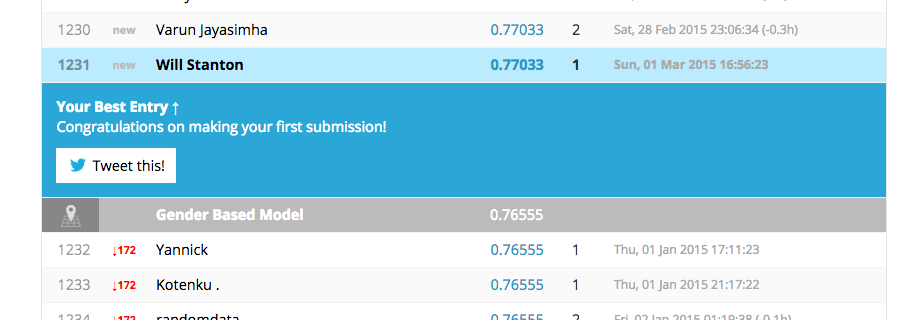
Uploading predictions is easy. Just go to the Kaggle page for the competition, click “Make a submission” on the sidebar, and select the file submission.csv. Click “Submit,” and then Kaggle will score your results on the test set.
Well, we didn't win, but we did pretty well. In fact, we beat several hundred other people and one of the benchmarks created by Kaggle! Our accuracy on the test set was 77%, which is pretty close to the cross-validation results of 82%. Not bad for our first model ever.
You can find the R code here.
This post only scratches the surface of what you can do with R and caret. Here are a few ideas for things to try in order to improve the model.
Okay, so you've done one machine learning classification tutorial and submitted a solution to Kaggle. That's an awesome start, and it's more than the vast majority of people ever do. So what's next? Here are a few things you can do: